psg_project
CS4641 Summer 2022 Project - Sleep Stage Classification
Andrew Inman, Ashok Iyer, Bryce Smith, Josh Lee
Infographic
Introduction
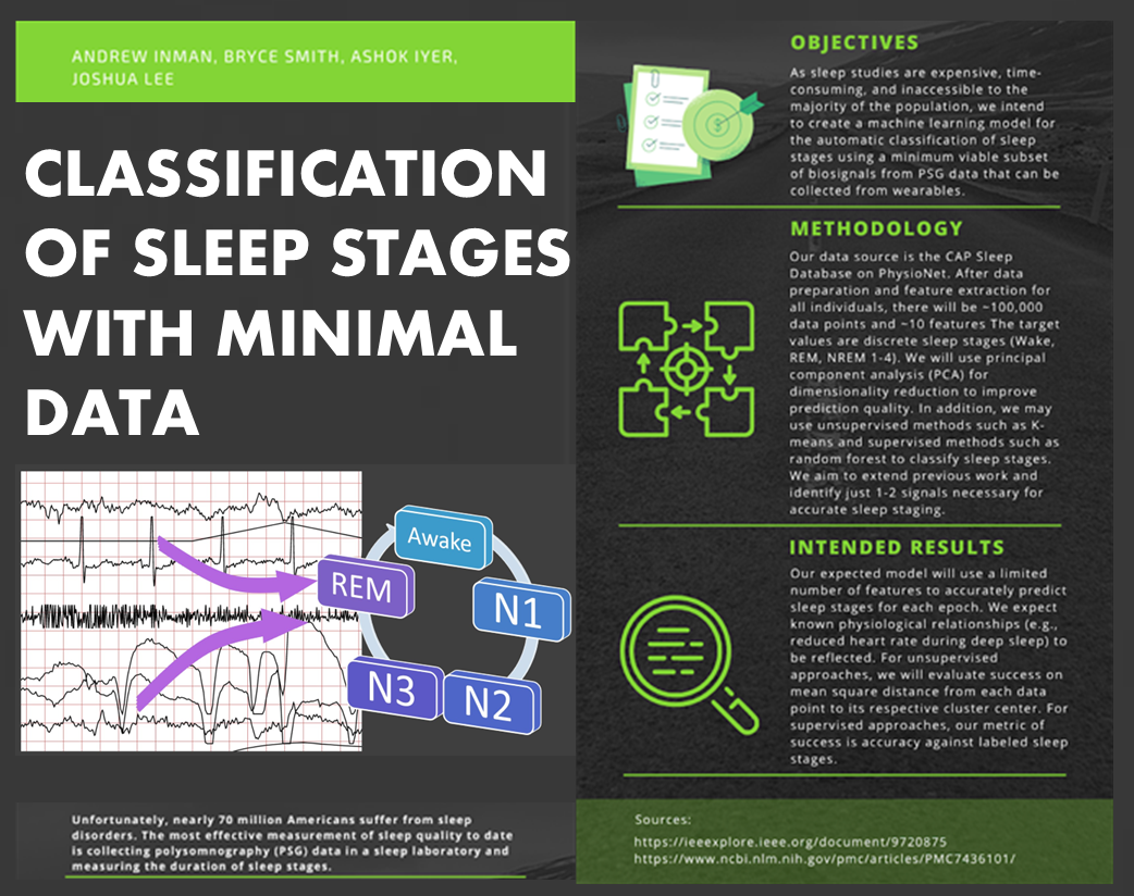
Sleep is an important physiological process directly correlated with physical health, mental well-being, and chronic disease risk. Unfortunately, nearly 70 million Americans suffer from sleep disorders.1 The most effective measurement of sleep quality to date is collecting polysomnography (PSG) data in a sleep laboratory and measuring the duration of sleep stages. However, sleep studies are expensive, time-consuming, and inaccessible to the majority of the population. Wearables have attempted to use heart rate data and machine learning algorithms to predict sleep stage, but suffer from low accuracy.2 We intend to create a machine learning model for the automatic classification of sleep stages using a minimum viable subset of biosignals from PSG data. Success of this algorithm could inform the design of and be applied in a simpler, more accessible sleep monitoring system that uses minimal sensors to accurately detect sleep stages.
Methodology
Dataset
Our data source is the CAP Sleep Database on PhysioNet.3 It contains PSG recordings for 108 individuals; each waveform has over 10 channels including EEGs (brain), EMGs (muscle), ECGs (heart), EOGs (eyes), and SAO2 (respiration) signals.4 From each voltage waveform we extracted numerical measurements taken every 1.9 milliseconds, generating a time series dataset. Additionally, for each individual, a text file provides labeled sleep stages every epoch (30 second interval) along with age, gender, and sleep disease information.
Due to significant variation in the exact signals recorded for each individual, we defined a common set of 11 signals found in most individuals: “Fp2-F4”, “F4-C4”, “C4-P4”, “P4-O2”, “C4-A1”, “ROC-LOC”, “EMG1-EMG2”, “ECG1-ECG2”, “DX1-DX2”, “SX1-SX2”, “PLETH”, and “SAO2”. The distribution of diseases in the 108 individuals is also very unbalanced, with only 16 “normal” individuals (no sleep disease), 2 individuals with Bruxism, 9 individuals with Narcolepsy, 40 individuals with NFLE (Nocturnal Frontal Lobe Epilepsy), 10 individuals with PLM (Periodic Leg Movement), 22 individuals with RBD (REM Behavior Disorder), and 4 individuals with SDB (Sleep-Disordered Breathing). Additionally, the number of individuals with useable data varies significantly within each of these disease groups. There is significant variation in the types of signals recorded in the “normal” individuals, and only 4/16 (25%) of them have all signals in the common set. Meanwhile, a majority of the individuals with NFLE, RBD, or PLM have all signals in the common set available. In order to select an overall balanced subset of individuals such that each disease has significant (not necessarily equal) representation while also trying to capture as much data as possible, we limited the number of individuals selected from these three groups such that no disease group had over 3 times as many individuals as another.
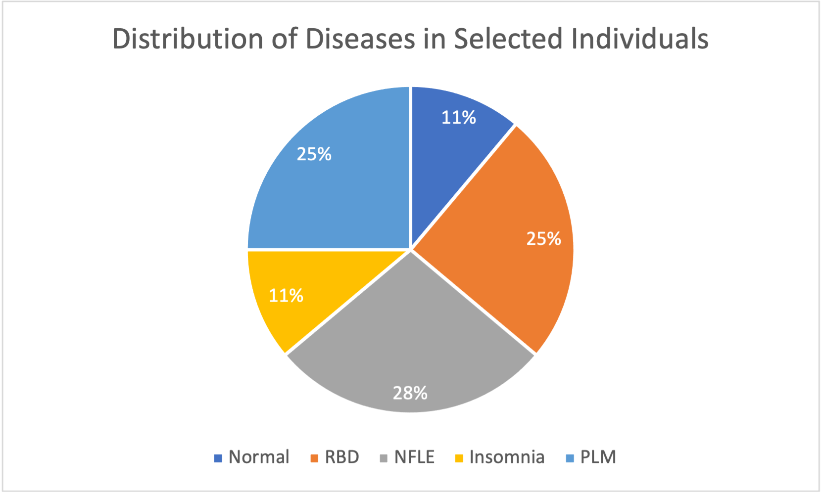
In total, 36 individuals were selected, with 4 normal individuals, 4 individuals with insomnia, 10 individuals with NFLE, 9 individuals with PLM, and 9 individuals with RBD. Narcolepsy, Bruxism, and SDB were not considered due to a lack of available data. From here, we divided these individuals into training and testing subgroups. Our training subset had a total of 22 individuals, with 2 normal individuals, 2 individuals with insomnia, 6 individuals with NFLE, 6 individuals with PLM, and 6 individuals with RBD. Our testing subset had a total of 14 individuals, with 2 normal individuals, 2 individuals with insomnia, 4 individuals with NFLE, 3 individuals with PLM, and 3 individuals with RBD. Our unsupervised learning methods exclusively used training data; we only added testing data for use in our supervised learning methods.
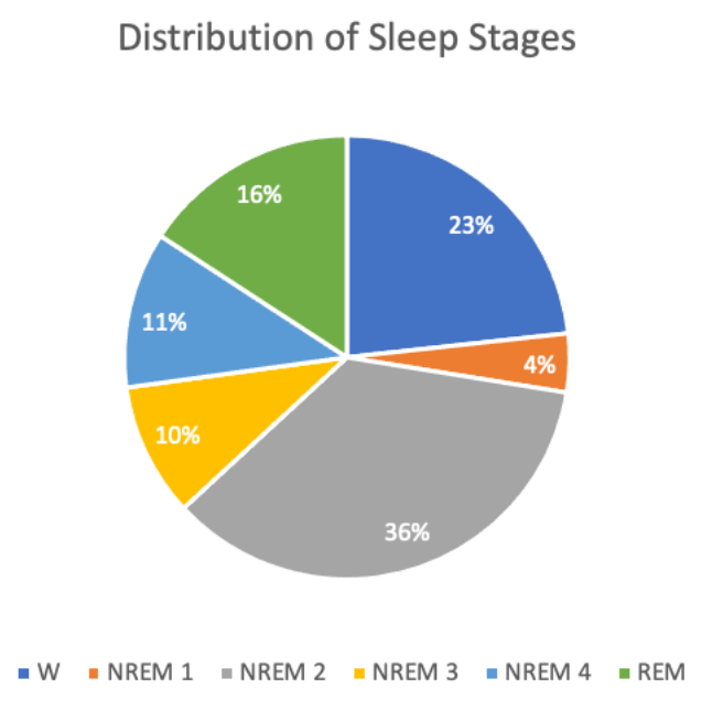
After data preparation and feature extraction for these individuals, there were ~30,000 total data points (~20,000 training, ~10,000 testing) and ~47 features, most of which were engineered. The target values are discrete sleep stages (Wake, REM, NREM 1-4). An overview of the distribution of sleep stages for all individuals in the dataset is shown below.
Data Preparation
Our initial data cleaning involved converting each individual’s waveform data to numerical measurements and capturing a common set of ~10 signals. The original data for each individual had a sampling frequency of 512 Hz, meaning measurements were taken every 1.9 milliseconds. However, the sleep stage labels provided for each individual were taken every 30 seconds. Therefore, we needed a way to encapsulate our original data into 30 second chunks in order to align PSG data with sleep stages. Simply averaging measurements across each epoch is not the best way to encapsulate the data for each epoch; we implemented feature extraction methods based on previous research on effective features for each type of signal to get multiple features from each signal. Feature Extraction methods are detailed below.
Due to physiological variability between PSG subjects, many of the recordings being taken years apart, and potential testing inconsistencies, such as electrode connection quality, there is high variability between the subjects’ baseline values. For example, the baseline EMG amplitude (background noise) for some subjects is significantly higher than others. Similarly, so subjects have a naturally higher heart rate than others. These differences in baselines are unique to each subject but persist through the entire recording. This was remedied by centering each individual’s data by subtracting the mean of each of their features before combining their data with the rest of the subjects’ data.
Outliers were detected in the dataset using the Local Outlier Factor (LOF) method. This algorithm considers if a point is an outlier among its nearest neighbors, as opposed to considering the point in relation to the entire dataset. Thus, extreme outliers due to recording errors are removed, but expected outliers, such as spikes in muscle activity are not removed. For example, when heart beats are overrun by noise due to recording abnormalities, certain heart rate metrics, such as the low frequency change in heart rate can spike, often by multiple orders of magnitude higher than expected. Such outliers were detected and removed based on the LOF method. Other statistical outliers, such as those due to spikes in EMG (muscle) activity are not removed using this method, which is advantageous because this type of outlier is a valid measurement that can be used to detect motion during sleep, often associated with REM and Wake sleep stages.
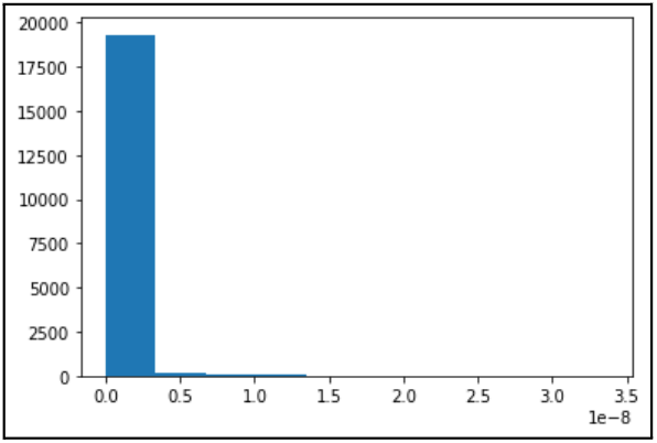
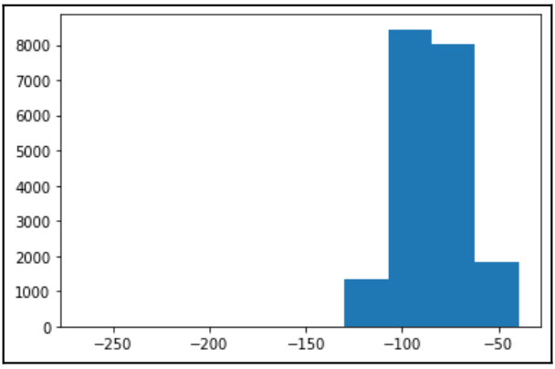
Finally, we applied robust scaling to our dataset using the interquartile range. We opted for robust scaling over standard scaling due to concerns regarding the effect of outliers on our dataset. The Box Cox Transformation was used to standardize all features to a normal distribution. The results of Box-Cox transformation applied to EOG Energy Content Band are shown below.
Before Box-Cox:
After Box-Cox:
Additionally, we used encoding methods to express sleep disease and sleep stage (target) in numerical form. For sleep disease, we employed “dummy” encoding; with five disease classes including “Normal”, we created four new binary variables that took value “1” if an individual had a certain disease and “0” if not, with a “Normal” individual having all four of these binary variables equal to 0. For sleep stage, we used “ordinal” encoding in which we simply assigned each sleep stage a numerical value; the “awake” stage was assigned value “0”, NREM stages 1-4 were assigned their respective stage numbers, and REM was assigned value “5”.
Feature Engineering
Feature extraction methods for each type of signal from the PSG data are described:
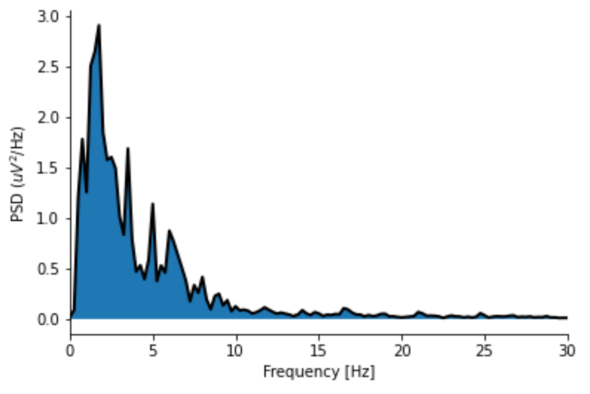
- EEG: EEG (electroencephalogram) is a technique used to detect electrical activity in the brain. Manual sleep stage classification is largely dependent on the fraction of brain waves with specific frequencies (e.g., delta waves with a frequency of 1 - 4 Hz) and secondary time-domain features. In our dataset, available EEG signals differ slightly between individuals, but broadly follow the International 10-20 System. Extensive literature exists on useful EEG features, so a subset of suggested features were selected. First, the time-domain EEG signal was decomposed into the frequency-domain using Welch’s method (see image below), and the power of each frequency band of each brain wave was computed. Second, multiple entropy-based metrics (i.e., metrics conveying the amount of information given by a signal) were computed. Finally, miscellaneous more sophisticated time-domain metrics (e.g., Petrosian fractal dimension) were calculated. In total, thirteen unique features were computed using the provided EEG signals. All EEG features were averaged across each individual’s EEG channels.
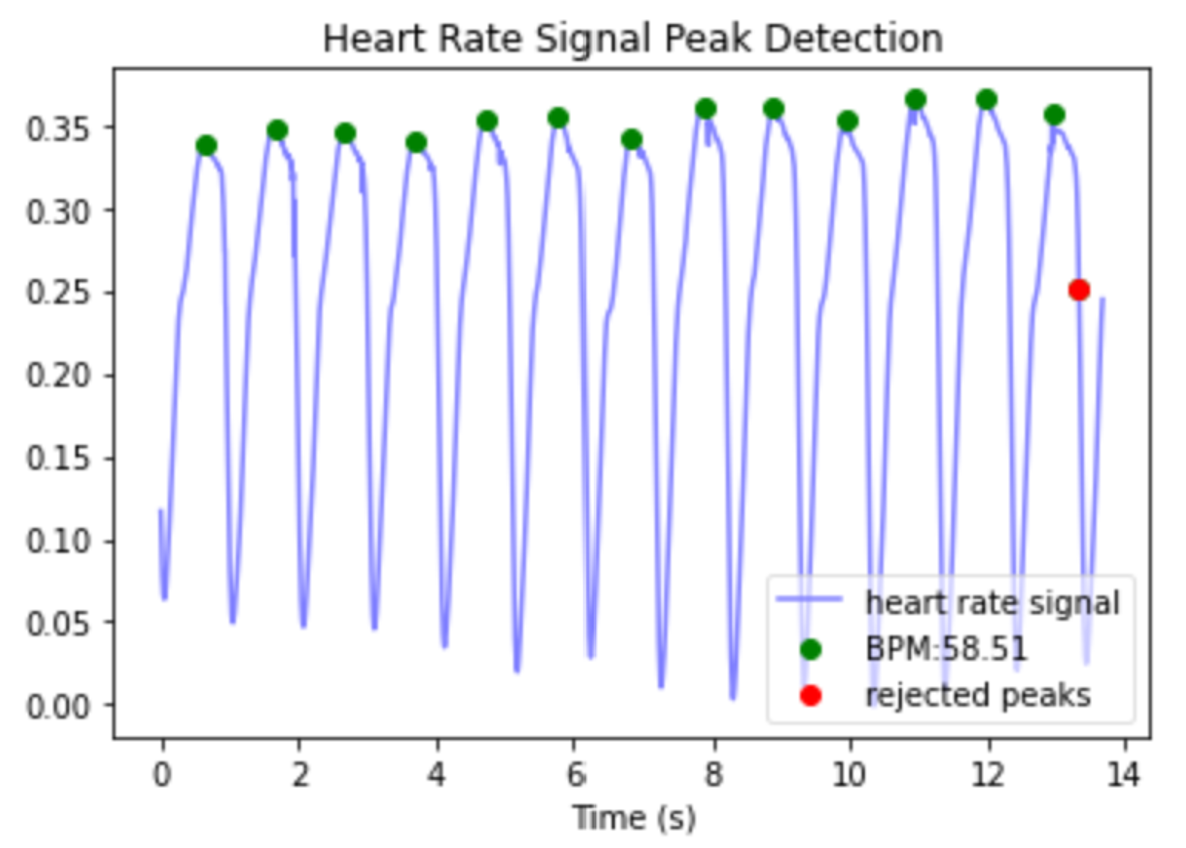
- ECG & PPG: ECG (electrocardiogram) and PPG (photoplethysmogram) are two methods used to record heart beats during the sleep studies. First, Python’s heartpy library was used to detect heart beats (see image below).5 Once heart beats were located, heart rate could be calculated. Beyond heart rate, an informative set of metrics consist of those that quantify variation in heart rate. The root mean square of the differences in time between adjacent heart beats (RMSSD) is one measure of heart rate variability, which is useful in our application because it can be meaningfully calculated over short time periods, such as 30 second epochs.6 Heart rate changes in the frequency domain, specifically “low frequency” changes (0.04-0.15Hz) and “high frequency” changes (0.15-0.5 Hz) have been observed to vary with sleep stage, so these were also applied using the implementation in the heartpy library.7,8
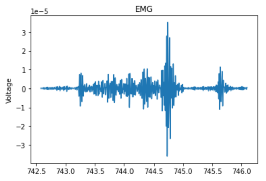
- EMG - EMG (electromyography) is a method for measuring electrical activity of muscles. The main metric used to quantify the EMG activity was energy, calculated as the sum of squared differences between each point and the sample mean, divided by the number of samples.9 Progression into deeper stages of sleep is typically correlated with a decrease in muscle tone, which corresponds to a decrease in baseline EMG energy, but REM sleep is also associated with brief spikes in muscle activity (see image below).10 To capture these transient spikes in EMG energy that were “averaged out” over an entire 30 second epoch, a moving average with a five second window was applied over each second, and the average of the five highest windows was recorded within each 30 second epoch.11
-
EOG: EOG (electrooculography) is used to detect activity within the human eye. One study aimed at Human-Computer Interaction applications mentioned a few useful features that were extracted from EOG signals, including: Maximum Peak Amplitude, which measures the maximum positive amplitude, Maximum Valley Amplitude, which measures the maximum negative amplitude, Area Under Curve, which is a summation of the absolute values of amplitude under positive and negative curves, and Signal Variance.12 All of these metrics were calculated within each epoch. Another study that focused specifically on sleep staging estimated the Power Spectrum for the EOG signal and calculated the Energy Content Band by integrating this function over the frequency range 0.35-0.5 Hz, where REM activity is concentrated.9 Using a Welch method to estimate the power spectrum, we calculated the Energy Content Band for each epoch.
-
SAO2: SAO2 (or SPO2) refers to a blood-oxygen saturation reading which indicates the percentage of hemoglobin molecules that are saturated with oxygen. Readings can vary from 0 to 100% . Normal reading will range from 94% to 100%. Literature suggests readings below 50% are artifacts. Related literature to sleep staging using oximetry data engineered features by taking the peaks of each time period and the percentage of time spent above a certain threshold.13 We followed suit with our data by taking the maximum of each epoch and the percentage of time spent above 70%, 80%, and 90% oxygen saturation by epoch. In addition, we included the average oxygen saturation of each epoch.
Feature Selection
After feature extraction, the correlation and mutual information methods were used to eliminate unnecessary features.
-
Correlation Method: Correlated features were detected and removed using the method proposed by Kuhn and Johnson.14 This method involves first calculating a correlation matrix for the data. Then, correlations are assessed pairwise. For any pair of features with a correlation above a set threshold (0.8 was used here), the feature in this pair with the larger average correlation between itself and every other feature was removed. This method eliminated 13 features, as shown in the results section.
-
Mutual Information Method: After using the correlation method, we calculated the normalized mutual information between each feature and the sleep stages (target values) and defined four feature sets: the top 5, 10, 20, and 30 features with the greatest normalized mutual information values. Ultimately, only the top 5 and top 10 sets have been used since they yield the strongest performance metrics.
Dimensionality Reduction
After feature selection, two methods were employed to reduce the dimensionality of data - Principal Component Analysis (PCA) and T-Distributed Stochastic Neighbor Embedding (TSNE). Broadly, PCA linearly transforms combinations of features such that variance is maximized along each principal component (i.e., axis). TSNE is a more sophisticated dimensionality reduction technique that is able to account for nonlinear features in data. Both techniques were employed on the four feature groups (i.e., top 5, 10, 20, & 30 features) and were used to reduce to 1, 2, 3, and 4 components. Isomap, a non-linear, manifold-based dimensionality reduction algorithm was also applied to the dataset. This algorithm differs from PCA in that it does not assume that datapoints that are close together in Euclidean space are meaningfully similar. Because the method did not yield noticeably improved differentiation of sleep stages in the reduced feature space compared to PCA, these results were not used with the unsupervised learning algorithms.
Unsupervised Learning
Following dimensionality reduction, we applied several unsupervised learning methods to our training data, including K-Means, GMM, and DBSCAN. To determine the quality of our clustering, we used the external measures of homogeneity, F1 score, normalized mutual information, Rand Statistic, and Fowlkes-Mallows measure. These external measures were selected because they quantify how clusters found by the unsupervised learning methods represent the known sleep stages (target values). Normalized mutual information was selected to quantify how much information we gather about our targets by knowing the unsupervised cluster assignments. The Rand Stat was applied to capture the accuracy of the cluster assignments. F1 and Fowlkes-Mallows were both selected because they represent both precision and recall. In our application, false positives and false negatives have similar impact, so a balance of precision and recall is desired. In order to calculate these clustering metrics, the sleep stages were taken as the “ground-truth” assignments, and each cluster was assigned a sleep stage based on the sleep stage of the majority of points in that cluster. We defined the “predicted” label of a point as the sleep stage of the cluster that it was assigned to.
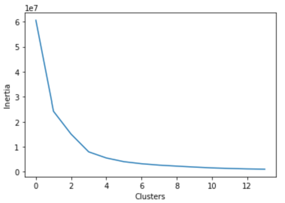
- K-Means: K-Means was applied to our dataset via the sklearn implementation. As K-Means is notoriously sensitive to outliers, we expected suboptimal results. Thus, we explored similar methods to K-Means such as K-Medians and K-Medoids which are both more resistant to outliers.15 K-Means gave the baseline behavior while K-Medoids was chosen as it was the most outlier resistant due to the nature of cluster center selection. We utilized the elbow method and found that 3 clusters was optimal for K-Means & K-Medoids (see image below). It should be noted that 6 clusters are expected for our dataset as this would capture each stage of sleep. Thus, we ran the K-Means & K-Medoids on both 3 and 6 clusters. Because the goal of our algorithm is to distiguish between all 6 sleep stages, the primary results shown here will be those achieved using 6 clusters. The Ancillary Results section shows K-Means applied with 3 clusters and a simplified interpretation of the sleep stages as Awake, NREM, and REM.
-
GMM: GMM was applied to our dataset via the sklearn implementation. Like K-Means, the most important parameter for GMM is the specified number of clusters. For our data, six clusters are used, corresponding to the 6 stages of sleep. The Ancillary Results section shows the performance of the algorithm when applied to only 3 clusters.
-
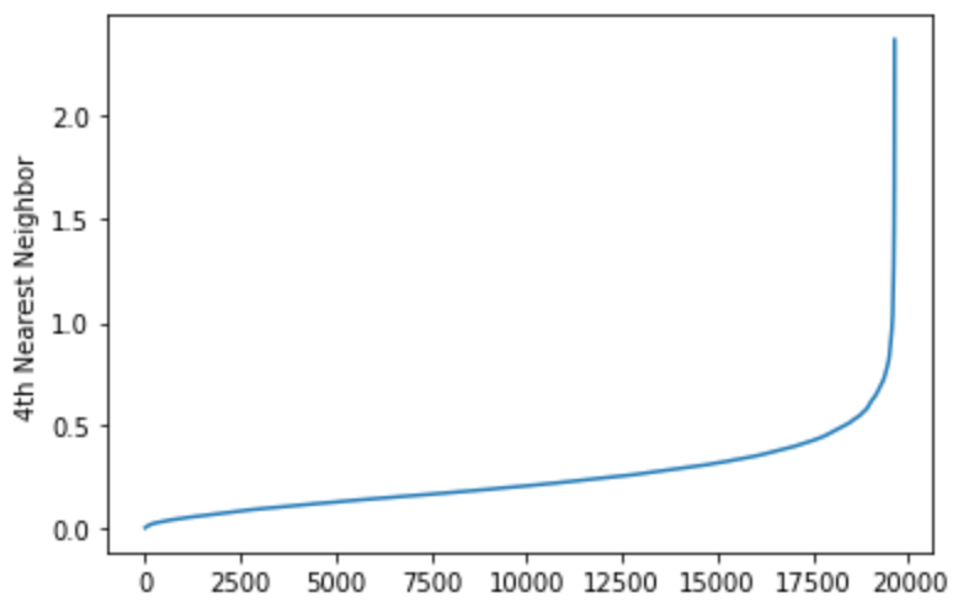
DBSCAN: DBSCAN was applied using the implementation in the sklearn package. The critical parameters to set for the algorithm are epsilon, or the maximum radius of a neighborhood around a point, and MinPts, the minimum number of points required to be in a point’s epsilon neighborhood for that point to be considered a core point. The starting value of MinPts was determined based on the dimensionality of the data being clustered, using the rule of thumb that in noisy datasets, a MinPts of 2xD is often appropriate. Epsilon was calculated using the distance to the 4 nearest neighbors of each point (see image below). These distances were sorted and plotted, yielding a graph that shows a flat region followed by a sharp increase in distance to outliers. A starting value of epsilon was selected as a value in the flat region of this graph, and it was adjusted further by steps of 0.1 to increase the clustering metrics.
Supervised Learning
Based on our unsupervised learning results and the imbalance in distribution of sleep stages, NREM stages 1-4 were consolidated into a single class before applying supervised learning algorithms. Many ML sleep staging studies, such as one by Satapathy16, build predictive models with a consolidated NREM class. This results in approximately 70% of datapoints having the target label ‘NREM’, which causes some algorithms to largely ignore the minority classes Wake and REM when making predictions in an attempt to optimize overall accuracy. Therefore, before running certain algorithms, undersampling and/or oversampling techniques were applied to our training data. This helps reduce artifical inflation of accuracy from data imbalances. Undersampling and oversampling techniques were applied after dimensionality reduction, and they were only applied to the training dataset. The supervised learning classification algorithms we applied include Naive Bayes, Logistic Regression, Random Forest, SVM, and LSTM Neural Network.
-
Undersampling: The undersampling technique used was the Neighborhood Cleaning Rule (NCR) as implemented in the Imbalanced Learn library. This technique assesses the nearest neighbors (3 neighbors were used) of each datapoint, and removes the data points for which all neighbors are not in the same class. In addition, NCR runs a 3 nearest neighbors classifier and removes data points not belonging to the predicted class.
-
Oversampling: The oversampling technique used was the Synthetic Minority Oversampling Technique (SMOTE). This method uses interpolation between data points in the same class to generate prototype data points for the class. This was used to add additional data points to the minority classes (Wake and REM) until they matched the number of points in the NREM class.
-
Naive Bayes: Gaussian Naive Bayes was applied using the implementation in sklearn. The best results were obtained by applying dimensionality reduction using a 5-component PCA and then isolating the 3rd, 4th, and 5th principal components. Following dimensionality reduction, one challenge in training an effective Naive Bayes classifier was overlapping data points from different classes. Even in regions that were primarily composed of a single sleep stage, there were often noisy data points from other sleep stages interspersed in these regions, so NCR undersampling was applied to clean these regions in the training dataset. The next challenge arose as a result of an imbalance between the relatively few REM data points and the more common Wake and NREM data points. SMOTE oversampling was applied following PCA to increase the number of the points in the minority classes.
-
Logistic Regression: Logistic regression was applied using the implementation in sklearn. The one-vs-rest technique was used to classify the data into three groups, and for each binary classification arising in the one-vs-rest comparisons, a probability threshold of 0.5 was used as the cutoff for predicting one class over another. As with the Naive Bayes classifier, prior to running the logistic regression, NCR undersampling and SMOTE oversampling were applied to the dimensionality reduced data.
-
Random Forest: After applying dimensionality reduction followed by undersampling to our training data using the Neighborhood Clearing Rule, Random Forest was applied to our dataset via the sklearn implementation. By default, the function fits 100 decision trees using a bootstrapping (random selection with replacement) of our training data and expands each tree until every node is pure. However, this expansion leads to major overfitting on our training data. One way to resolve this issue is through pruning, which eliminates certain branches of the node at the cost of greater impurity of nodes. Adjusting the ccp_alpha parameter in the sklearn implementation is one method of pruning. Using the sklearn default of 100 trees, we can determine the optimal ccp_alpha by finding the lowest value that maximizes prediction accuracy in our testing data. The plots below show parameter tuning using our top 5 dataset after applying a two-dimensional TSNE algorithm.
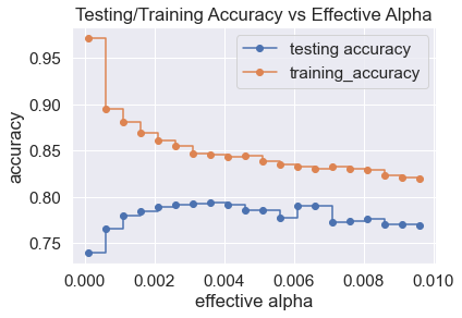
Based on the plot above, the optimal ccp_alpha value is 0.0035. Random Forests of various sizes were fitted to our training data and their prediction accuracies on testing data were checked to determine an appropriate number of trees.
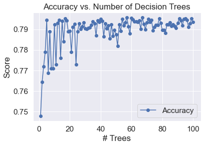
Based on the plot above, prediction accuracy stabilizes significantly as the size of a Random Forest increases. Since the prediction accuracy is mostly stable for Random Forests comprised of over 50 decision trees, a forest of 100 decision trees is appropriate.
Another parameter that is often tuned in Random Forest is the number of features used in each decision tree, but this was not found to be helpful in improving accuracy for the top 5 data after a two-dimensional TSNE, which is logical given the small dimensionality.
-
SVM with Linear Kernel: Support vector machines are robust, supervised models commonly used for classification and regression of labeled data. A support vector machine with a linear kernel was applied to the dataset across after applying PCA dimensionality reduction for 1 - 5 features. No undersampling or oversampling was used. Based on unsupervised learning results, this technique was only applied to PCA results from the Top 5 and Top 10 feature sets. Additionally, the same training and testing sets were used as preceding supervised learning techniques. Finally, accuracy and the F1 metric were compared across PCA features and between the Top 5 and Top 10 feature sets. Furthermore, confusion matrices were used to compare performance.
-
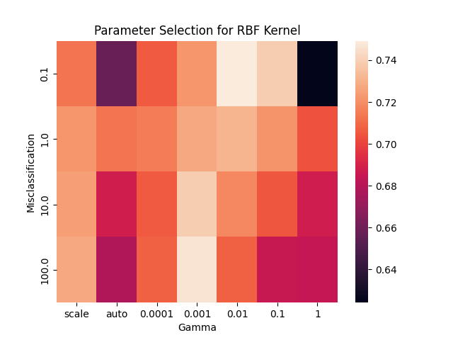
SVM with RBF Kernel: A support vector machine with a radial basis function (RBF) kernel was applied to the dataset after TSNE dimensionality reduction to two dimensions. This was completed both with and without NCR undersampling and SMOTE oversampling. The parameters for SVM with the RBF kernel are a misclassification term, C, which allows for more misclassification at lower values, and gamma, the positive coefficient of the exponent in the RBF kernel function. In order to set these parameters, a grid search was performed. This involved testing every combination of these parameters over a specified range (C from 0.1 to 100 and gamma from 0.0001 to 1). For each parameter combination, a 5-fold cross validation was performed, and the combination achieving the best accuracy was selected. A heat map showing the accuracy acheived with each parameter combination is whosn below. During this grid search, only the designated training data was used. The selected parameters were then used to apply the SVM model to the designated testing data, and slight adjustments were made manually to further improve accuracy.
-
LSTM Neural Network: This implementation of a recurrent neural network utilizes the continuous changes to the biases and weights of the network with respect to certain aspects of the previous data that has been processed. Epochs, learning rate, and the number of hidden layers were tuned to develop the most optimal model that we could muster. In addition, we experimented with adding different convolutional and pooling layers as per related literature. The changes to the model failed to improve the model due to overfitting. Our final hyper-parameters were as follows: batch size-1, hidden layers-2, epochs-1000, learning rate-0.001, and a ReLu activation function. Adam was used as our optimization algorithm. Our data was processed by TSNE with 2 components.
-
MLP Neural Network: After applying dimensionality reduction followed by undersampling to our training data using the Neighborhood Clearing Rule, a Multi-Layer Perceptron (MLP) neural network was applied using the sklearn implementation. Experimenting with the various parameters of the function, such as activation function, number of hidden layers, number of neurons in each layer, type of weight optimization solver, and regularization term size did not result in a consistent noticeable improvement in accuracy or F1 score. As a result, the model fitted on the data used the default variables provided in the sklearn function, which includes a ReLU hidden layer activation function, 1 hidden layer with 100 neurons, and a regularization term of 0.0001. The weight optimization solver used was stochastic gradient descent based.
Results
Feature Engineering & Selection
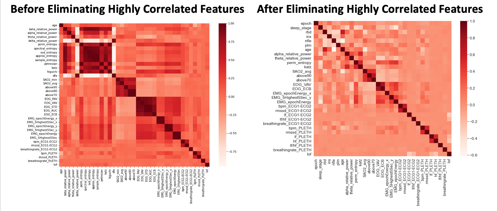
The feature engineering and selection process discussed in the Methodology section was followed. As discussed, we selected the top 5, 10, 20, and 30 features and consider these sets separate for dimensionality reduction & unsupervised learning tasks. As an example, the image of the correlation matrix below shows the original 37 features (left) being reduced to a set of the 30 features with the lowest correlation and highest mutual information (right).
- Figure 1: Correlation Heat Map Before and After Eliminating Highly Correlated Features
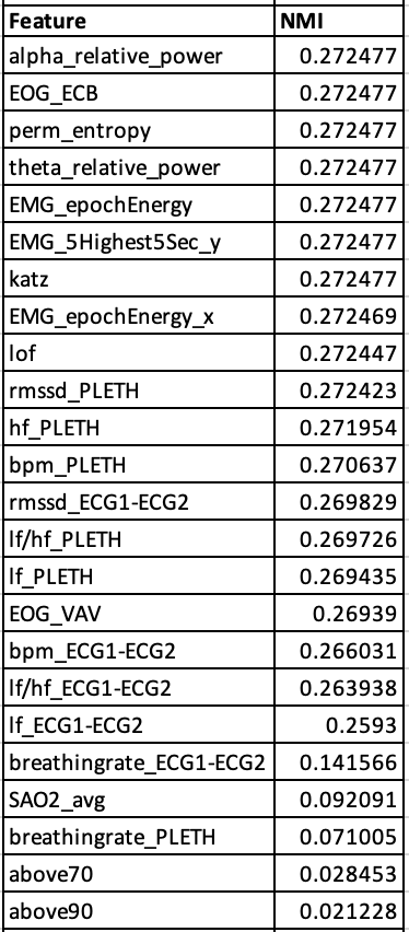
After removing highly correlated features, normalized mutual information with the target values (sleep stages) was calculated, and the most informative features were selected.
- Figure 2: Remaining Features Sorted by Normalized Mutual Information Values
Dimensionality Reduction
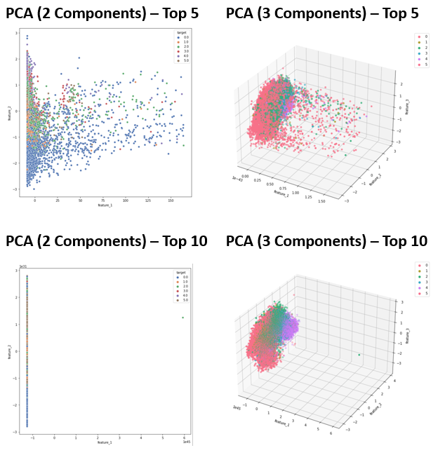
The dimensionality reduction process using PCA and TSNE described in the Methodology section was followed. The results of dimensionality reduction when reducing the top 5 and top 10 features to 2-3 dimensions is shown below.
- Figure 3: PCA Results - Training Data
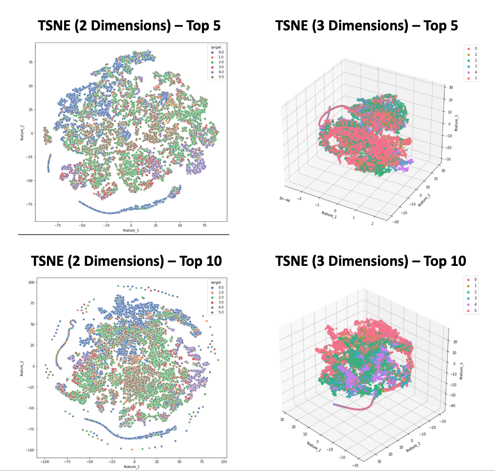
- Figure 4: TSNE Results - Training Data
Isomap dimensionality reduction was also applied to the data. Because the results did not yield greater differentiation of the sleep stages than PCA and presented the added difficulties of a mixture of low density and high density regions and abnormally shaped clusters, these results were not put through the unsupervised learning algorithms.
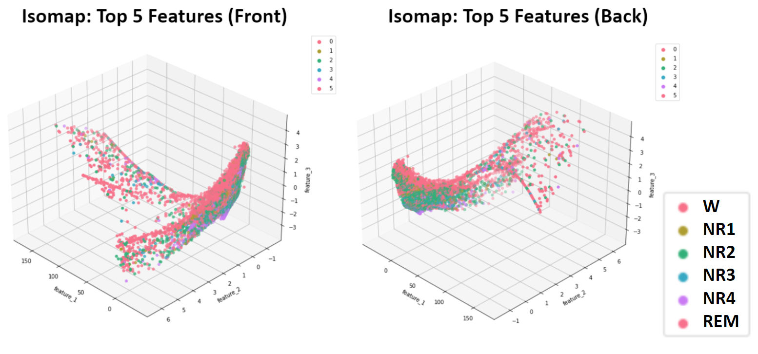
- Figure 5: Isomap Dimensionality Reduction of 5 Top Features - Training Data
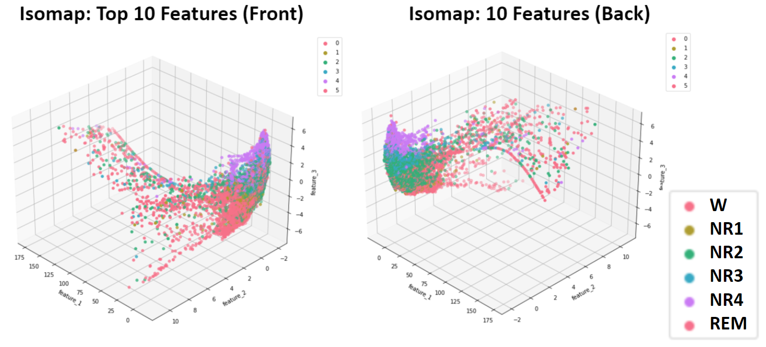
- Figure 6: Isomap Dimensionality Reduction of 10 Top Features - Training Data
Unsupervised Learning
After dimensionality reduction, K-Means, GMM, and DBSCAN were implemented on our training data according to the process outlined in the Methodology section. All of the algorithms performed best on the Top 10 feature sets, so only these results are provided. Although each algorithm was applied to each number of reduced components, only the best results are shared here: K-Means (3rd & 4th PCA components), GMM (3rd & 4th PCA components), and DBSCAN (3 TSNE Components).
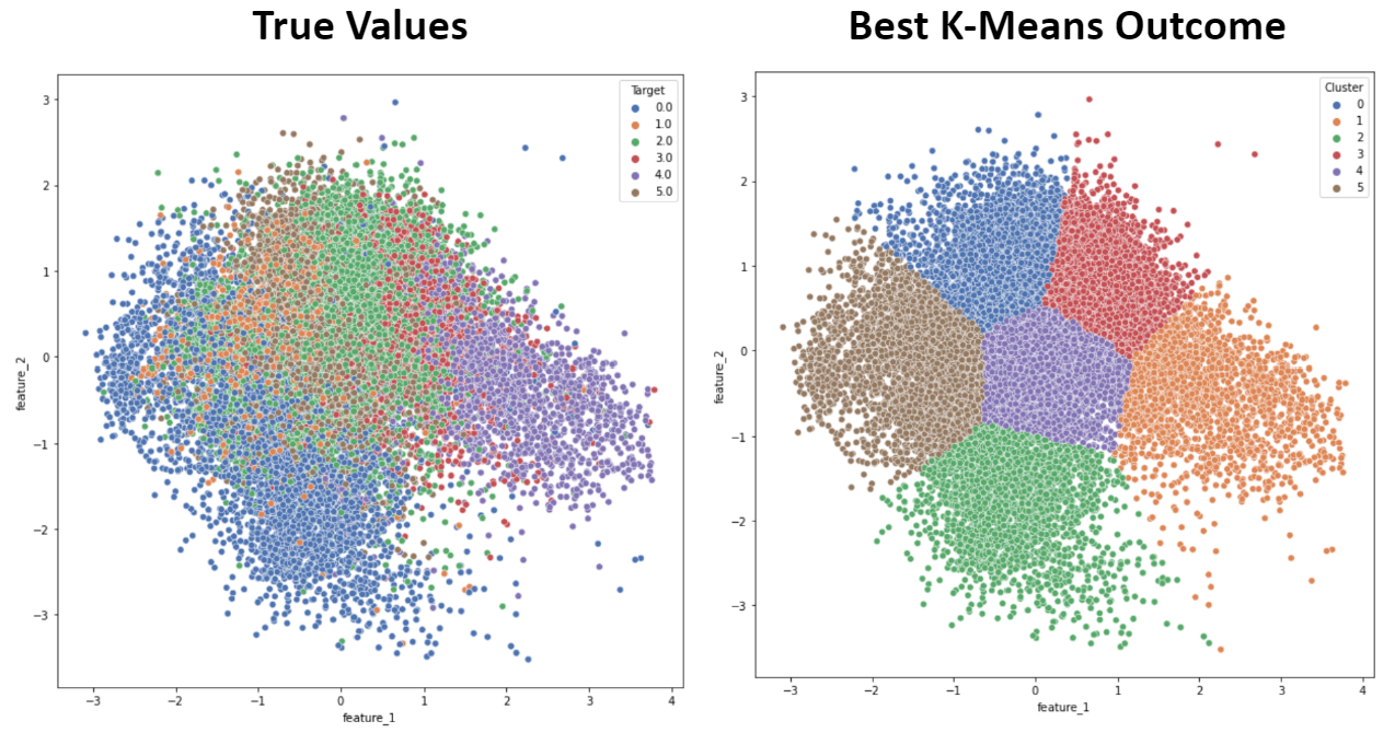
- Figure 7: K-Means Best Outcome
- Figure 8: GMM Best Outcome
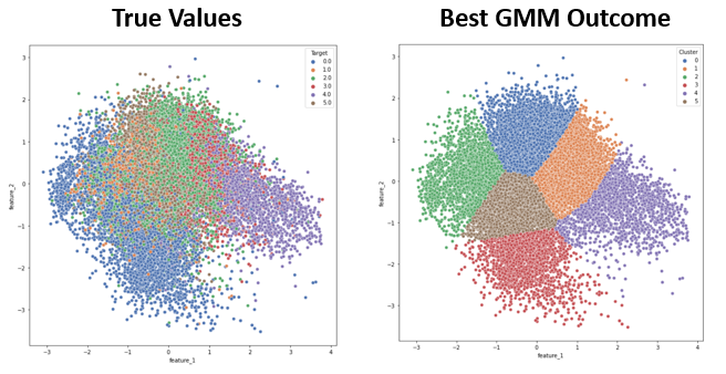
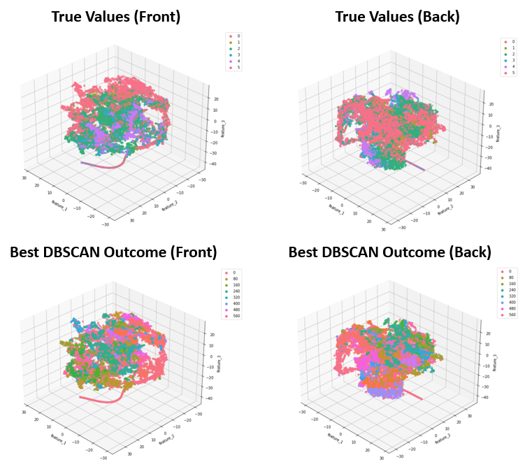
- Figure 9: DBSCAN Best Outcome
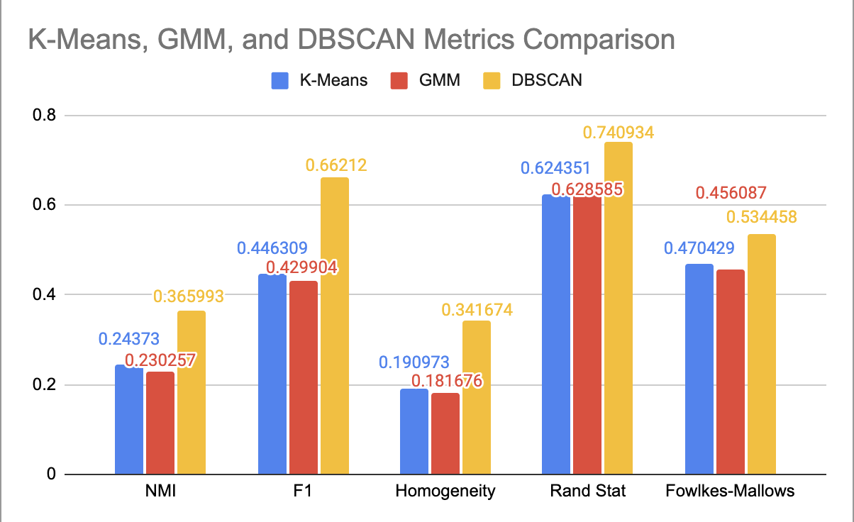
The external quality measures for the best result of each algorithm are provided in the bar plot below.
- Figure 10: Comparison of Performance for Each Clustering Algorithm
Simplification of K-Means and GMM Clustering
As mentioned, applying the elbow method for K-Means suggested an ideal cluster size of 3. Because the six sleep stage targets present in this dataset (Wake, NREM1, NREM2, NREM3, NREM4, and REM) can be more broadly grouped into only three more general targets (Wake, NREM, and REM), K-Means and GMM with three clusters were applied and compared to these broader sleep stage classifications. Wake points were given the label 0, NREM points were given the label 1, and REM points were given the label 2. Due to the improvement in metrics, this grouping was also employed for supervised learning algorithms.
- Figure 11: K-Means - 3 Target Values
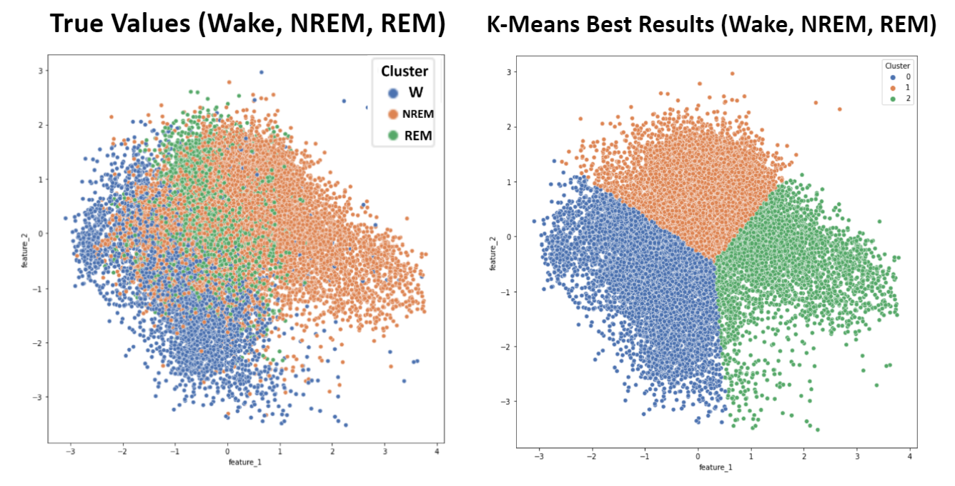
- Figure 12: GMM - 3 Target Values
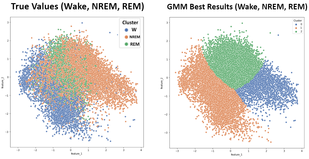
- Table 1: Clustering Metrics - 3 Target Values
| NMI | F1 | Homogeneity | Rand-Stat | Fowlkes-Mallows | |
|---|---|---|---|---|---|
| K-Means | 0.2303 | 0.8074 | 0.2515 | 0.6750 | 0.7297 |
| GMM | 0.2940 | 0.8282 | 0.3227 | 0.7013 | 0.7509 |
Supervised Learning
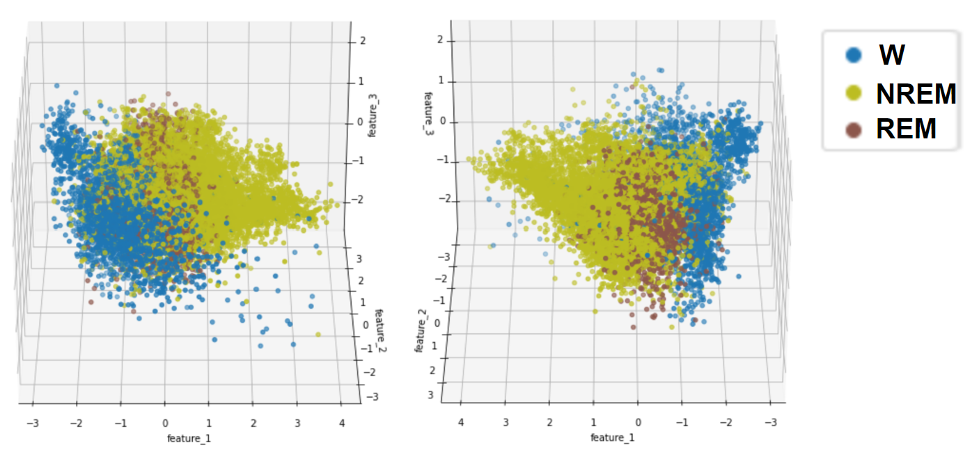
- Figure 13: Target Values for Naive Bayes and Logistic Regression
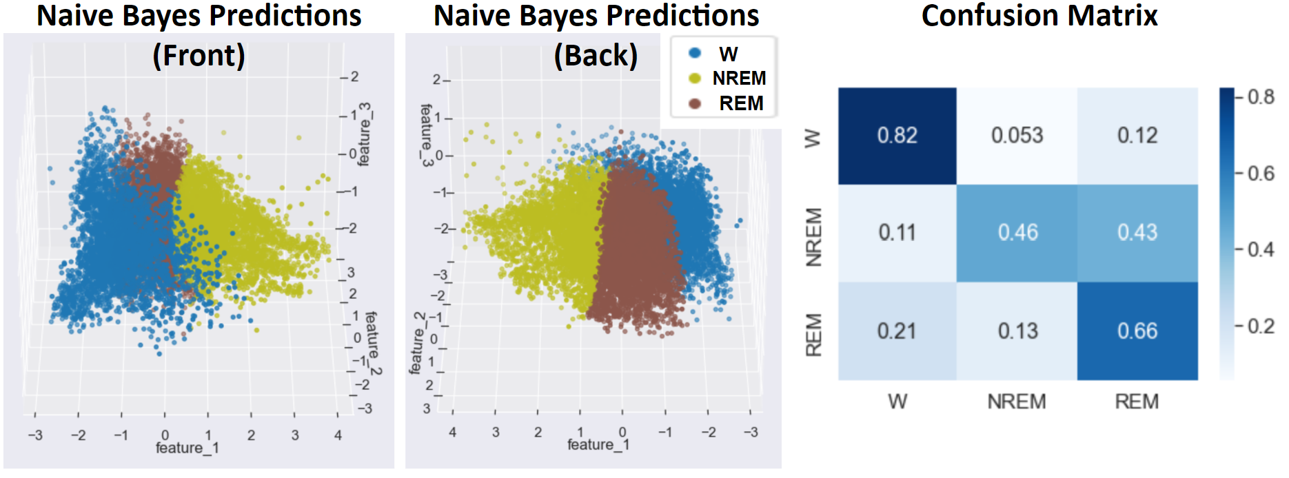
- Figure 14: Naive Bayes Best Outcome
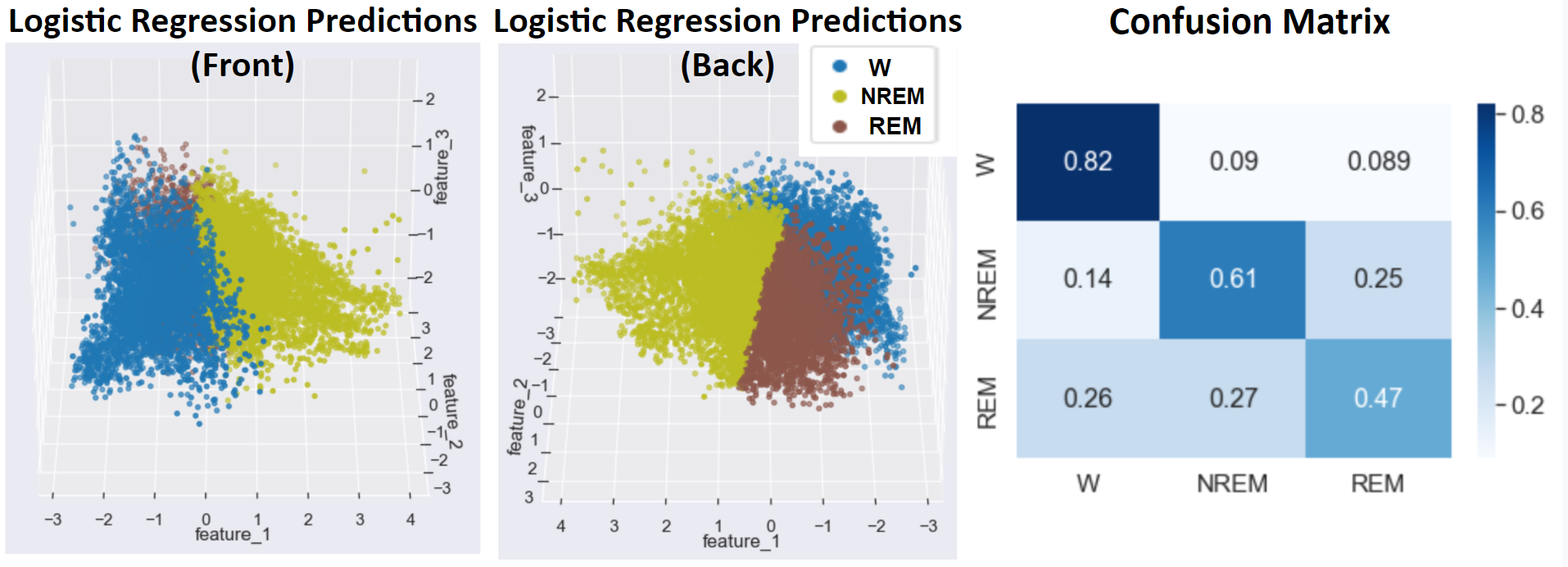
- Figure 15: Logistic Regression Best Outcome
- Figure 16: Random Forest Best Outcome
- Figure 17: SVM with Linear Kernel Best Outcome
- Note: Points in plot are Testing data points. Shading shows SVM decision boundaries.
- Figure 18: SVM with RBF Kernel
- Figure 19: SVM with RBF Kernel after Undersampling and Oversampling
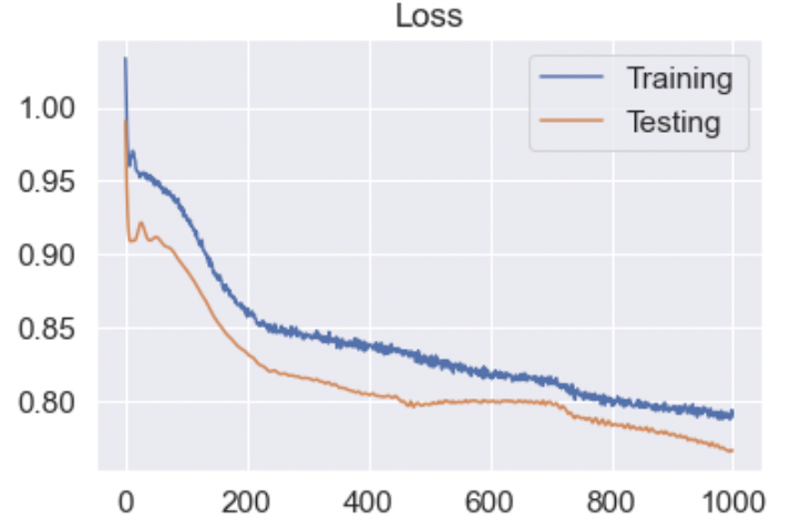
- Figure 20: LSTM Best Outcome
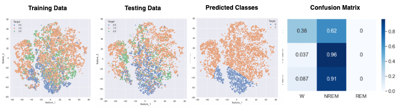
- Figure 21: LSTM Loss
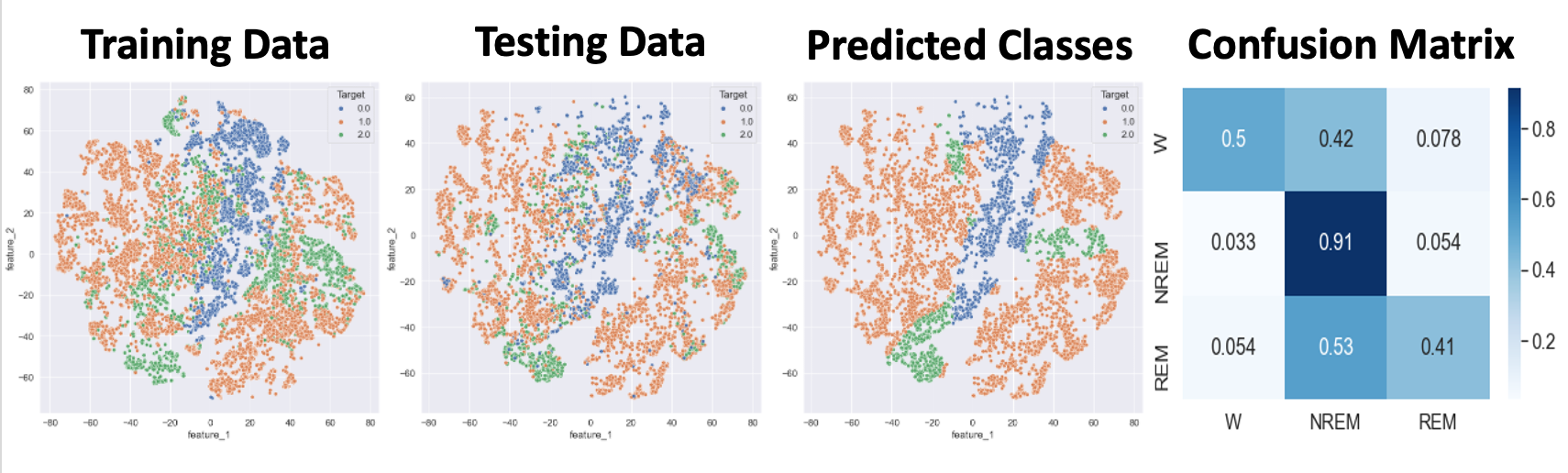
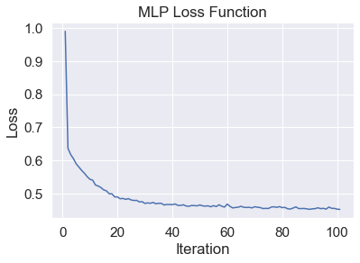
- Figure 22: MLP Best Outcome
- Figure 23: MLP Loss
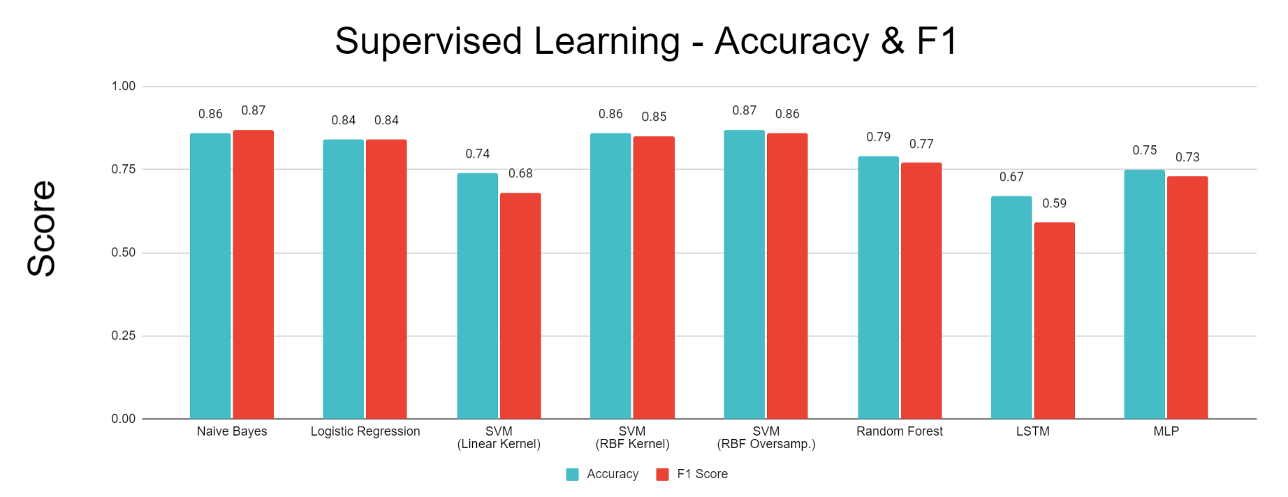
- Figure 24: Comparison of Performance for Each Classification Algorithm
Discussion
Note: All figures referenced are defined in the Results section.
Distribution of Targets & Important Features
Based on the pie chart in the Methodology section showing distribution of target values, the most frequent sleep stage in our data is NREM stage 2, but other stages like W (awake) and NREM stage 4 also comprise significant proportions. The class imbalance here may have contributed to poor results with our unsupervised learning methods. Since NREM stage 2 is the most prevalent sleep stage, most clusters will likely be assigned NREM stage 2 as well based on our definition. This means the predicted label of points in those clusters will also be NREM stage 2, but there is still a significant likelihood that a good portion of these points correspond to other sleep stages.
The histograms in the Methodology section compare overall EOG energy content band data before and after Box-Cox transformation. As evidenced by Figure 2, EOG energy content band has one of the highest normalized mutual information scores with sleep stage labels, making it an important feature, and it reflects the extreme right skewness that most other features in our dataset exhibit. However, we see that the Box-Cox transformation makes the distribution significantly more normal-shaped. Standardizing the shape of all features through Box-Cox transformation allows the data to be more balanced and reduces the impact of outliers.
Feature Engineering & Selection
As evidenced by the left image in Figure 1, there was high correlation among features within the same domain, especially EEG and EOG. For example, the EOG metrics AUC (area under curve) and STD (standard deviation) were closely correlated (correlation = 0.99). This is likely because AUC is the sum of the absolute values of individual voltage values in an epoch, so when AUC is higher, this indicates that there were more spikes in the EOG signal, causing the measurements to be further spread out overall. Similarly, two EMG metrics were used to measure EMG energy, which corresponds to muscle activity. One metric was an average EMG energy across an entire 30 second epoch, while the other was generated using a moving average with a 5 second window and then averaging the five highest 5 second periods. Although this second metric is more sensitive to spikes in EMG activity, across most epochs, it was very closely correlated with the average across the entire epoch (correlation = 0.97). As a whole, co-linearity between features in this dataset can be explained by similarity in the feature extraction calculations used to generate metrics for the same signal type. These closely correlated features do not add significant insights to the model, so they can be removed to simplify the model. Beyond simplification, removing these correlated features within signal domains can improve the performance of later algorithms, such as PCA, by reducing imbalanced impacts on variance resulting from the uneven number of features used for each type of signal. Following removal of the thirteen features identified during this step, the dataset had much lower correlation overall, as seen in the right image in Figure 1, in which there are no large regions of highly correlated data that would skew PCA and other algorithms.
Due to the high correlation between features within these domains, most of the features removed via our average correlation threshold were EEG and EOG features. We selected different sets of features with the top 5-30 normalized mutual information values with sleep stages for comparison purposes, since one of our project goals is determining a minimum viable subset of signals that can be used for accurate predictions. The features that had the lowest mutual information with sleep stages were Oxygen Saturation metrics, which is surprising given that breathing rate is known to decrease during deep sleep. We applied two stages of feature extraction in order to avoid issues with high-dimensional data like overfitting and distorted distance calculations in clustering. For example, the EMG metrics for the 5 second moving average and the 30 second epoch average were closely correlated (correlation = 0.97), so the moving 5 second average was removed because of the two metrics, it had a higher average correlation across all other features (average correlation = 0.3418). From there the EMG epoch average moved on to the mutual information feature selection step where it was removed from the set of “Top 5” features because it had the seventh highest mutual information with sleep stage.
Dimensionality Reduction
We investigated two primary dimensionality reduction algorithms, PCA and TSNE. In our results from PCA, shown in Figure 3, outliers cause variance to be highly concentrated in the first principal component, leading to a tight distribution of data points in others. This can be observed in Figure 3, in which the majority of data points appear “flattened” onto one axis or plane, corresponding to the lower-variance components. This issue becomes more apparent when we increase the dimensionality of the dataset, as evidenced by comparing the PCA results from the Top 5 versus Top 10 feature sets. When we examine the target values of points across the entire first principal component in these plots, we see that most are in the “awake” stage since most of the spread-out points correspond to spikes in signals, such as muscle activity, which are most common when someone is awake.
We also implemented TSNE, as the algorithm better accounts for nonlinear relationships in our data. For optimal performance, sklearn recommends that TSNE be applied to a dataset with less than 50 features; given that we have 5 to 30 features, TSNE appears to be a viable method for our data. Figure 4 shows the output obtained from TSNE. The spread of data points is higher than PCA results, but the data points still tend to be tightly distributed with significant overlap between points corresponding to different sleep stages. The clear presence of outliers and irregularly shaped clusters indicate that after applying TSNE, DBSCAN will have much better performance than K-Means or GMM.
Isomap was also implemented. The most notable general trend across the Top 5 and Top 10 datasets (Figures 5 and 6) was one dense cluster with a gradient corresponding with target sleep stage. Coming off of this cluster are “tendrils” that largely correspond to the Wake stages and likely separate from the main cluster due to inclusion of outliers. Because these results suffer from both inconsistent densities as well as irregularly shaped cluster, the unserpervised methods that follow were not applied to these Isomap dimensionality reduction results.
Unsupervised Learning
For the purposes of this project, since we are looking at the accuracy of predicting sleep stage, supervised metrics using target values as “ground truth” is the most logical method of evaluating the quality of our clustering. The use of internal measures is not useful unless each cluster clearly corresponds to a distinct sleep stage, which is not the case.
The bar chart comparing external metrics between unsupervised learning approaches, shown in Figure 10, provides insight into algorithm performance. All of the metrics shown in the chart range from 0 to 1, with higher values indicating better clustering performance. The results from K-Means and GMM are extremely close, with K-Means performing slightly better in all metrics with the exception of the Rand-Stat. Since the metrics for DBSCAN are all greater than for K-Means and GMM, we can conclude that our best DBSCAN outcome seems to be the best clustering for our data. However, there seems to be a positive correlation between each metric value for the different algorithms; the metrics that have higher values for one algorithm also tend to have higher values for the other. For all three algorithms, the metric with the highest value is Rand-Stat and the metric with the lowest value is Homogeneity.
All of our clustering algorithms run into issues due to the tight distribution of points in reduced dimensionality. The reduced dimensionality from both PCA and TNSE looks very compact, with a lot of overlap between points corresponding to different sleep stages. As mentioned earlier, periodic outliers are common in our data. This may explain why K-means did not perform very well in general, since it is especially sensitive to outliers, and the best results were achieved by effectively removing these outliers by dropping the first principal compononts. The sleep stage clusters appear to have highly irregular shapes, which is difficult for both K-means and GMM to categorize. Further, although a gradient in sleep stage can be observed in the True Values of Figures 7 and 8, unsupervised metrics such as K-Means and GMM are based on the general assumption that points in the same cluster are close to eachother and far away from other clusters. This is not the case in this PCA dimensionality reduction, and the overlap between different sleep stages makes it challenging for these algorithms to detect clear boundaries between clusters. Instead, the clusters simply converge on regions within the large PCA cluster, which results in inaccurate classification and very low cluster purity (Low homogeneity) because each cluster contains many points from other sleep stages.
Interestingly, K-Means and GMM had very similar performance when applied on the 3rd and 4th components of a 4D PCA with our top 10 dataset. Our PCA results indicate that the vast majority of data variance is concentrated within the first principal component, leaving much less in the others. Therefore, by isolating these components, we can focus on data with very low variance. As variance approaches zero, GMM converges to K-Means, which can explain the similarity in results.
Due to the irregularly shaped clusters resulting from the TSNE dimensionality reduction, DBSCAN was the most suitable clustering algorithm to apply to the TSNE dimensions. The best results, shown in Figure 9, were achieved by applying DBSCAN to a three-dimensional TSNE dimensionality reduction. Although relatively high values were achieved for the clustering metrics, especially the Rand Stat (0.74), Fowlkes-Mallows (0.53), and F1 measures (0.66), these results were only achieved by setting a low enough epsilon that all of the small clusters in the TSNE feature space could be captured as unique clusters by the DBSCAN algorithm. This helps with the purity and accuracy of each cluster, but the downside is an uninterpretable cluster assignment of ten clusters to describe only six sleep stages. This clustering result will therefore have poor generalizability to other datasets, and would require knowing the target values in order to interpret the large number of clusters as capturing one sleep stage or another, ultimately defeating the purpose of this being an unsupervised method that could be meaningfully applied without have access to the data labels. On the other hand, the results from GMM and K-Means, while not as good based on our selected metrics, are potentially more interpretable because the PCA dimensionality reduction that they are applied to shows more of a gradient from one sleep stage to the next. So even without known sleep stages, clusters could be reasonable assigned to sleep stages by following this gradient.
Sleep stage prediction seems to be more tailored towards supervised learning methods. Most machine learning projects on sleep staging have gone directly to supervised learning algorithms with great accuracy. Part of our objective in applying unsupervised learning was to take a novel approach and evaluate the viability of unsupervised learning methods for this problem. Assigning each cluster the “majority” sleep stage is not an accurate way to summarize clusters since, as evidenced by the dimensionality reduction plots, there is significant overlap between data points with different sleep stage labels. Another potentially significant issue is that there is not enough distinction between different NREM stages. Machine learning projects that deal with sleep staging often focus on classifying awake, REM, and NREM sleep since there is a lot of overlap in the metrics corresponding to the different stages of NREM sleep, which are often difficult to distinguish based on metrics extracted from PSG data. Indeed, improved results for both K-Means and GMM were observed by simplifying the classification problem to one with only Awake, NREM, and REM labels. Additionally, the proportion of individual NREM sleep stages in our data is significantly uneven. The significant overlap between data points from different sleep stages may be attributable to our pooling of individuals with different diseases. Individuals with different sleeping disorders may present different sleeping characteristics, such as abnormal EEG signal for individuals with noctural frontal lobe epilepsy, or increased EMG activity for those with periodic limb movement (PLM).
Supervised Learning
We relied primarily on accuracy and F1 scores to evaluate our supervised learning methods. There is no preference between “False Positives” and “False Negatives” in sleep stage predictions. The primary focus is on maximizing “True” predictions, which are encompassed by the accuracy score calculation. F1 is another measure commonly used to evaluate the success of classification algorithms, and provides equal importance to “False Positives” and “False Negatives”.
In the sleep staging study by Satapathy, Random Forest achieved the best accuracy among several supervised learning methods.16 However, the study includes comparisons with others that used methods like SVM and Bayesian classifiers which yielded comparable accuracy.16 We employed all three of these methods with the addition of Logistic Regression for an additional comparison along with MLP and LSTM Neural Networks due to their potential to produce highly-accurate predictive models.
Compared to more advanced methods, such as Random Forest, SVM, and an LSTM neural network, Gaussian Naive Bayes with the addition of NCR undersampling followed by SMOTE oversampling achieved high accuracy and F1 measures at 86% and 87%, respectively, and higher accuracies in the confusion matrix in the Wake and REM stages. This method likely outperformed many of the more advanced methods due to the noisy and overlapping nature of PSG signals. Because many of these signals, such as oxygen saturation, heart rate, and brain waves are maintained by the body within a relatively small range that allows the patient to stay alive and asleep, there is significant overlap of these signals in different sleep stages, as can be seen in the overlapping regions of each sleep stage in Figure 13. This overlapping data coupled with the noise inherent to data collected from biosignals result in a high potential for supervised classifiers to overfit to noisy data. Because a Gaussian Naive Bayes classifier was used, the decision boundaries learned from the training data do not take on the complex curvature of RBF Kernel SVM or the jagged shape of a decision tree’s boundary. As a result, the Naive Bayes classifier is less susceptible to overfitting to noisy data points, giving it impressive accuracy compared to the more complex methods that can capture more detail but tend towards overfitting. Another advantage of Naive Bayes comes from its improved accuracy in predicting the Wake and REM sleep stages that have fewer data points when coupled with undersampling and oversampling. Applying NCR undersampling before training the Naive Bayes classifier helps to remove overlapping, noisy data points, thus preventing SMOTE from oversampling non-representative data points. Because oversampling the Wake and REM stages directly increases the prior probability of these classes, the posterior probability used to classify these stages also increases. As a result, the Naive Bayes classifier responds well to oversampling by directly increasing the probability of classifying a datapoint as one of the less prominent sleep stages, REM or Wake. This causes the relatively high accuracy in these stages seen in the confusion matrix of Figure 14, which results in increasing the overall accuracy and F1 scores.
Much like Gaussian Naive Bayes, Logistic Regression achieved an accuracy of 84%, relatively high compared to many of the more advanced supervised methods. As in the Naive Bayes classifier, combining Logistic Regression with undersampling and oversampling helped to improve the accuracy of classifying the sleep stages with fewer available data points in the original dataset. Specifically, the Wake stage was predicted very accurately by this model, as seen in the confusion matrix of Figure 15, helping to increase the overall accuracy. Also, similar to Naive Bayes, Logistic Regression prevented overfitting by learning planar decision boundaries that are less susceptible to the overfitting made possible by methods like Kernel SVM, decision trees, and neural networks that learn decision boundaries containing more complex curvature or jagged, highly variable separators.
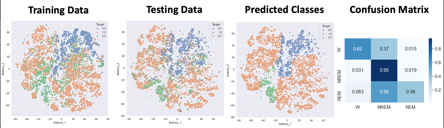
Figure 16 shows the best results with Random Forest, which uses the top 5 data after applying a two-dimensional TSNE algorithm. This prediction achieved high scores of 79% accuracy and 77% F1. The training and testing data plots in Figure 15 appear to have similar patterns of sleep stage distribution, with the datapoints labeled “Wake” (0) concentrated in the upper right area, the datapoints labeled “REM” (2) concentrated in the lower left area, and the NREM datapoints concentrated in the upper left and lower right areas. Visually, the decision lines appear to be quite similar. This is validated by the fact that before any pruning (ccp_alpha value of 0), the prediction accuracy is close to 75%, as shown in the corresponding plot in the “Methodology” section. While the lack of pruning certainly leads to overfitting of decision trees on the training data, the loss in accuracy due to this overfitting is not very large because of the similar boundaries, and the introduction of pruning improves the generalizability of the decision lines even further. The plot of predicted classes in Figure 15 closely follows these general patterns. Based on the confusion matrix, a vast majority of the NREM datapoints were predicted correctly; in the other two classes, many of the datapoints were incorrectly predicted as belonging to NREM, especially REM points. This can be explained by the fact that in our training data, while the points belonging to REM tend to be concentrated in the lower left area, a significant number are also found in other areas that overlap significantly with the other two classes. Meanwhile, the points belonging to the other two classes, especially NREM, are more exclusively concentrated in certain areas with less overlap elsewhere, and NREM points anyway make up the greatest proportion of the training data even after undersampling. The predicted classes plot shows that our random forest completely ignores any REM points outside of the lower left region, which hinders the accuracy in that class because of how many REM points overlap with other regions along with the fact that there are fewer REM points to begin with.
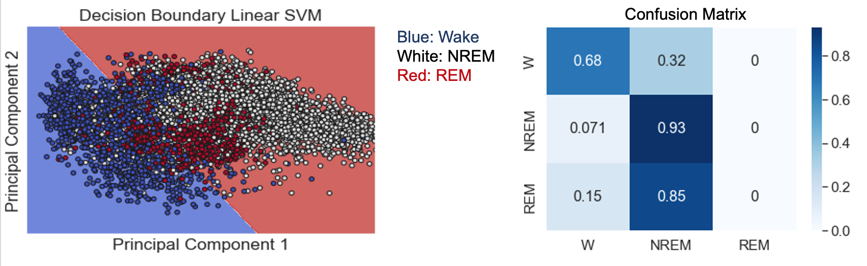
The best performance for the support vector machine using a linear kernel was obtained when applying PCA (with 5 components) to the Top 5 Features, as shown in Figure 17. This model had an accuracy of 74% and an F1 metric of 68%. However, while the model is able to differentiate between “Awake” and “NREM” with modest accuracy, the confusion matrix reveals that it is unable to identify “REM” sleep. Looking at the decision boundary, it can be observed that the “REM” sleep stage is interspersed with “Awake” and “NREM” points. It is recommended that undersampling with a nonlinear kernel is used to improve model accuracy in the future.
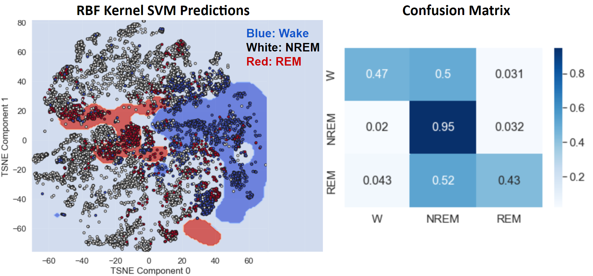
SVM with a radial basis function kernel achieved an accuracy of 86% and an F1 score of 85%. This method improved upon the accuracy of the linear SVM because the RBF kernel allows for a decision boundary with complex curvature to be learned. As a result, this method could be successfully applied to the TSNE dimensionality reduction, which does a better job of separating the sleep stages than PCA but generates abnormal shapes that are not suited to linear SVM. As seen in Figure 18, the RBF kernel enabled the decision boundaries to generally follow the non-linear arrangement of the different sleep stages within the 2-dimensional TSNE space. Also, because the SVM was applied with a regularization term, the model allowed some points to be misclassified, helping to avoid overfitting and reduce the effects of noise on the model. One problem with this method is that although the RBF kernel allowed the model to capture all three sleep stages, it still suffered from a relatively unbalanced accuracy in detecting each sleep stage. The confusion matrix in Figure 18 shows that the model correctly classified the NREM stage at a much higher rate than the REM and Wake stages. This is problematic because the NREM stage is the majority class in the dataset, so high accuracy in predicting this class leads to a high overall accuracy, but the model’s utility is limited if it only predicts one sleep stage accurately.
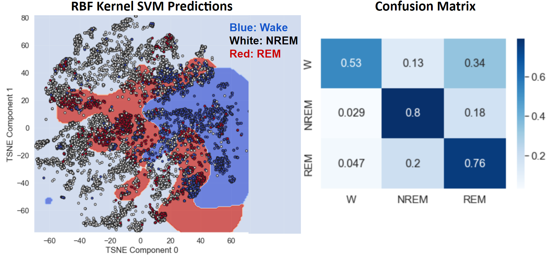
To address the imbalanced accuracy of the RBF Kernel SVM, the model was learned after applying NCR undersampling and SMOTE oversampling to the TSNE output. The overall accuracy of 87% and F1 score of 86% remained approximately the same as RBF SVM without these techniques, but the model was more balanced in its accuracy across all three sleep stages, as seen in the confusion matrix of Figure 19. This improvement comes from the fact that oversampling enabled smaller groups of data points in minority classes to have a stronger effect on the learned decision boundary. As a result, the regions defining REM and Wake in the oversampled model are larger and more contiguous, enabling more points from these stages to be correctly classified. This comes at the cost of higher misclassification of NREM data points, but this tradeoff is beneficial because there is more value in a sleep staging model that can discern all sleep stages with reasonable accuracy than in a model that can only detect one sleep stage.
Figure 20 displays the performance of the LSTM network, which used the top 10 data after applying a two-dimenstional TSNE algorithm. This prediction acheived 67% accuracy and 59% F1 . Our network failed to identify REM points in our dataset. As seen in Figure 20, REM points lacks a clearly defined border as opposed to NREM and Awake points. This is the most likely cause for the model’s failure to recognize these points. Figure 21 displays the loss of the model during training. A consistent trend between the two curves displays a lack of overfitting with our datasets. Figure 22 shows the best results with an MLP Neural Network, which uses the top 5 data after applying a two-dimensional TSNE algorithm. This prediction achieved 74% accuracy and 73% F1. Unlike LSTM, MLP does not completely ignore REM points, which explains why it performs better.
In order to improve performance any further, we will likely need to train our models with more data.
References
- Malekzadeh M, Hajibabaee P, Heidari M, Berlin B. Review of Deep Learning Methods for Automated Sleep Staging. 2022:0080-0086.
- de Zambotti M, Goldstone A, Claudatos S, Colrain IM, Baker FC. A validation study of Fitbit Charge 2™ compared with polysomnography in adults. Chronobiology International. 2018/04/03 2018;35(4):465-476. doi:10.1080/07420528.2017.1413578
- Goldberger AL, Amaral LAN, Glass L, Hausdorff JM, Ivanov PCh, Mark RG, Mietus JE, Moody GB, Peng C-K, Stanley HE. PhysioBank, PhysioToolkit, and PhysioNet: Components of a New Research Resource for Complex Physiologic Signals. Circulation 101(23):e215-e220 [Circulation Electronic Pages; http://circ.ahajournals.org/content/101/23/e215.full]; 2000 (June 13).
- Terzano MG, Parrino L, Sherieri A, et al. Atlas, rules, and recording techniques for the scoring of cyclic alternating pattern (CAP) in human sleep. Sleep Med. Nov 2001;2(6):537-53. doi:10.1016/s1389-9457(01)00149-6
- van Gent P, Farah H, van Nes N, van Arem B. HeartPy: A novel heart rate algorithm for the analysis of noisy signals. Transportation Research Part F: Traffic Psychology and Behaviour. 2019/10/01/ 2019;66:368-378. doi:https://doi.org/10.1016/j.trf.2019.09.015
- Shaffer, F., & Ginsberg, J. P. (2017). An Overview of Heart Rate Variability Metrics and Norms. Frontiers in public health, 5, 258. https://doi.org/10.3389/fpubh.2017.00258
- Vanoli E, Adamson PB, Ba-Lin n, Pinna GD, Lazzara R, Orr WC. Heart Rate Variability During Specific Sleep Stages. Circulation. 1995/04/01 1995;91(7):1918-1922. doi:10.1161/01.CIR.91.7.1918
- Boudreau P, Yeh WH, Dumont GA, Boivin DB. Circadian variation of heart rate variability across sleep stages. Sleep. 2013;36(12):1919-1928. Published 2013 Dec 1. doi:10.5665/sleep.3230
- E. Estrada, H. Nazeran, J. Barragan, J. R. Burk, E. A. Lucas and K. Behbehani, “EOG and EMG: Two Important Switches in Automatic Sleep Stage Classification,” 2006 International Conference of the IEEE Engineering in Medicine and Biology Society, 2006, pp. 2458-2461, doi: 10.1109/IEMBS.2006.260075.
- Gonzalez AA, Rezvan, Kaveh, Valladares, Edwin, Hammond, Terese. Sleep Stage Scoring. Medscape. 2019;doi:https://emedicine.medscape.com/article/1188142-overview#a3
- Levendowski DJ, St Louis EK, Strambi LF, Galbiati A, Westbrook P, Berka C. Comparison of EMG power during sleep from the submental and frontalis muscles. Nat Sci Sleep. 2018;10:431-437. Published 2018 Dec 6. doi:10.2147/NSS.S189167
- S. Aungsakul, A. Phinyomark, P. Phukpattaranont, C. Limsakul, Evaluating Feature Extraction Methods of Electrooculography (EOG) Signal for Human-Computer Interface, Procedia Engineering, Volume 32, 2012, Pages 246-252, ISSN 1877-7058, https://doi.org/10.1016/j.proeng.2012.01.1264.
- Choi, E., Park, D.-H., Yu, J.-H., Ryu, S.-H., & Ha, J.-H. (2016, November). The severity of sleep disordered breathing induces different decrease in the oxygen saturation during rapid eye movement and non-rapid eye movement sleep. Psychiatry investigation.
- Kuhn, M., Johnson, K. (2013). Data Pre-processing. In: Applied Predictive Modeling. Springer, New York, NY. https://doi.org/10.1007/978-1-4614-6849-3_3
- Clustering with KMEDOIDS and common-nearest-neighbors¶. scikit. (n.d.).
- Satapathy S, Loganathan D, Kondaveeti HK, Rath R. Performance analysis of machine learning algorithms on automated sleep staging feature sets. CAAI Transactions on Intelligence Technology. 2021;6(2):155-174. doi:https://doi.org/10.1049/cit2.12042